3D Deep Learning for Perception

3D Deep Learning is the area of machine learning on 3D data. Typically 3D data comes from sensor measurements like LiDAR, radar, stereo-camera, etc. Due to the wide applications of point cloud data like computer vision, robotics and autonomous systems it has gained a lot of attention recently. Tasks like 3D shape classification, 3D detection and tracking and 3D segmentation are very common in above mentioned areas.

Due to the success of deep learning on images/2d data, the area of 3d deep learning grows. By simply naively applying 2d vision techniques on 3d data uncovers unique challenges which will be mentioned in this blog post.

Why use 3D data instead of just images?

3D data provides rich geometric, shape, scale and depth information. 2D Images lack those informations because of missing depth information. It is quite challenging extracting with certainty depth information out of images, although works like depth anything looks quite promising. Still cameras will have limitations working in edge cases and are extremely vulnerable to light, weather and seasonal challenges. This is empirically proven in autonomous driving scenarios where camery-only perception lacks robustness in conditions like fog, rain, snow etc. Still camera provides dense data with very good color and texture information which is very valuable. One additional thing: Cameras are very cheap!!! On the contrary point clouds coming from LiDAR are not affected by weather or light conditions and provide accurate depth information. The downside is that LiDAR’s are extremely costly, being around $10^4-10^5$ $.

3D Data Characteristics

Point clouds are a $set$ of points in the Euclidean space which is represented as $P_i=\mathbb{R}^{N \times (3+C)}$ where $N$ is the number of points, 3 stands for $x,y,z$ coordinate and $C$ denotes additional features like reflection intensity, etc.

The following characteristics make it quite challenging naively applying typical network architectures to point clouds:

• Permutation invariance

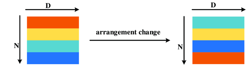
Permutation or order invariance refers to the characteristic that the order doesn’t matter at all for the point cloud. The above image would output the same point cloud no matter the order, that is why point clouds are a $set$ of points. Our network should also be “permutation” invariant. When we think about RNN’s or CNN’s, those models are NOT permutation invariant because the order indeed matters.

• Irregular/Sparse

Taking a look at LiDAR the point clouds are typically quite dense near the LiDAR but will become increasingly sparse in far distance. Either our network should be able to work with sparse point clouds or we’ll need a preprocessing step for point cloud completion (which is another network filling in multiple new points to make the point cloud dense).

• Invariant to rigid transformation Rotating, translating, reflecting or scaling point clouds should not affect our predictions thus making it invariant to the global coordinate system the point clouds are represented w.r.t.

• Interaction between points A single point has no value to us. For classification we care about global features, for segmentation we care about local and global features of the point cloud.

3D Data Characteristics

The first step in designing neural networks is to think about the data representation. There are multiple ways to represent 3D Data which has its own advantages and disadvantages. Depending on the representation type we will choose different models to fit the data.

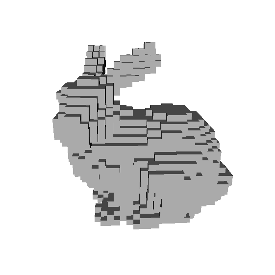
Voxels

Voxels discretize the space of point clouds into regular predefined 3D grids being $(d_w, d_h, d_l)$. They are equivalent to pixels in images, so voxels are regular and structural, so we can apply 3D Convolutions to learn features. Voxels use TSDF (Truncated Signed Distance Function) to represent 3D surfaces, where it restricts the values between $+1,-1$ . Whenever we have points inside a voxel it is denoted as 1 and outside as -1. And there is also one problem with voxels. Typically point clouds are sparse and irregular distributed therefore a lot of voxels will be empty. In practical applications there are sparse convolutions, which will be covered later. Voxels are extremely memory inefficient as they grow with cubic memory $O(n^3)$ where $n$ is the number of voxels. This is also a tradeoff you have to take. Whenever you want a more finegrained representation of the 3D data, you have to use small voxel size. But a small voxel size will result in a lot more voxels and therefore more computational memory. The choice of the right voxel size is quite challenging. We do not want to lose to much information due to the quantization process. An advantage of voxels is that they can summarize a complex 3d scene into regular grids and obtain good global representation. One can also apply 3D convolutions to voxels. In recent papers it is empirically shown that voxels are particularly good for large objects.

Another representation which can be also viewed as voxels are pillars. Pillars are just voxels with infinity height so they are defined as $(d_w, d_h = \infty, d_l)$. This representation quantizes the space even more than voxels.

BEV

Birds Eye View is a dense 2D representation, which can be obtained from either voxels or pillars where the 3D representation is projected to 2D. Another method for obtaining BEV is summarizing points statistics (binary occupancy, height and density of local point cloud).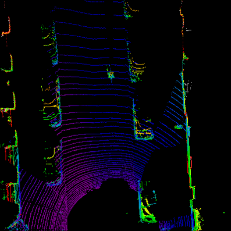

3D Deep Learning on raw point clouds

One of the pioneering work on deep learning on point clouds is PointNet (https://arxiv.org/pdf/1612.00593.pdf). Let’s dive deeper how PointNet is designed to fulfill the requirements and characteristics mentioned above.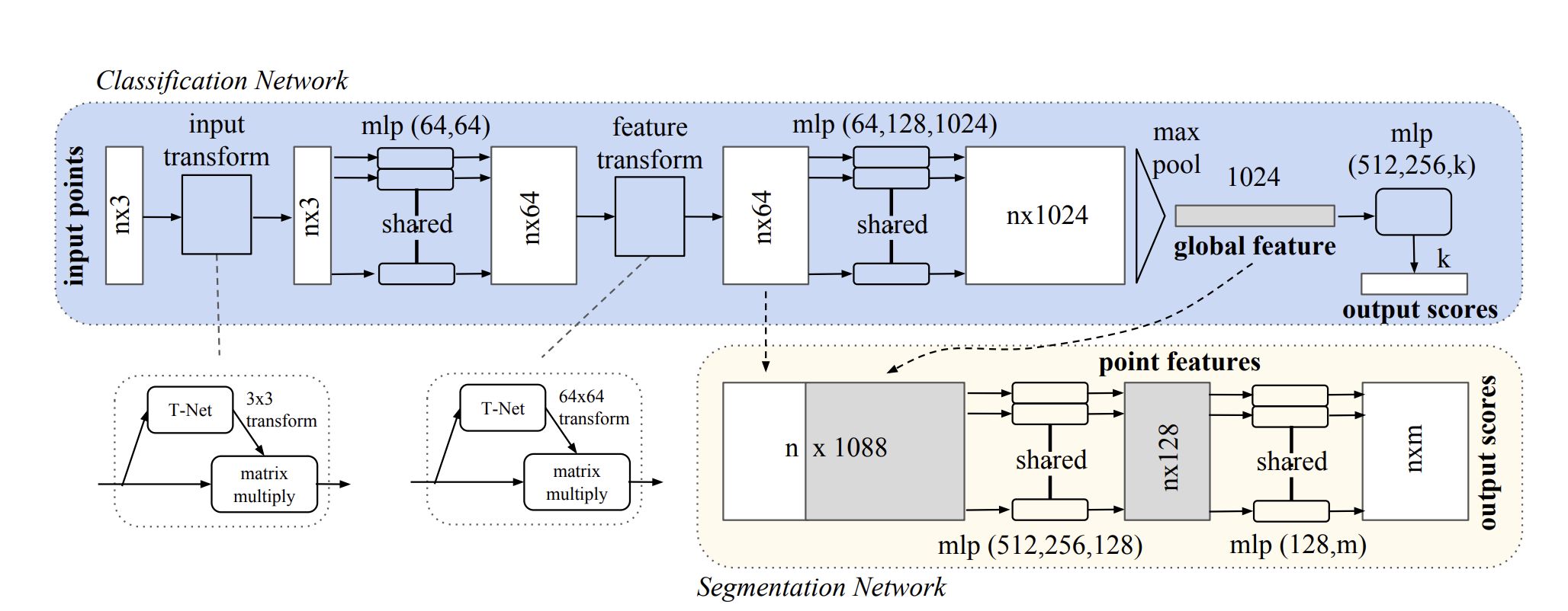

Permutation invariance: the authors of PointNet did introduce a symmetric function to make it invariant to permutations. The following functions are symmetric and invariant to permutations:

• $sum(a_1, a_2, …, a_n) = sum(a_n, …, a_2, a_1)$
• $max(a_1, a_2, …, a_n) = max(a_n, …, a_2, a_1)$

The authors use specifically max-pooling in the last layer before classification to aggregate the global features from the inputs. The output dimension of 1024 is fixed as MLP’s expect the same dimension no matter the number of points. The global feature vector is directly used for classification as we are interested in the global representation of the point clouds and disregard the local features of it (Same as in 2D CNN classification we do not care about the local low-level semantic features).

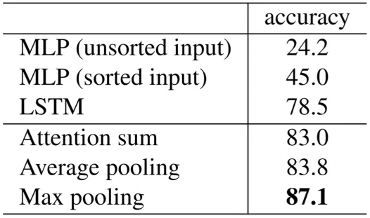
Authors have empirically tried other feature aggregation methods, but Max Pooling seems to be working the best. How I try to think about the global feature is that for every point n in our point cloud the max pooling extracts the feature which is most activated out of 1024 possible features. And every feature describes different local properties (the word local is pretty important for PointNet) of the specific point in the point cloud. One feature could be where in the euclidean space the point is located.

The invariance to rigid transformation is achieved in the T-Net modules (Joint Alignment Network as named by the authors). What the T-Net is doing. The T-Net is inspired by Spatial Transformer Networks which learns pose normalization given an input to transform it to canonical space. Because in Point Clouds the points could be permuted, rotated, scaled etc. in an infinit number of ways, the authors of PointNet adapt STN to lower the complexity of learning and the need of multiple data augmentations to “mimic” the unnormalized input. Instead of learning it implicitly, we can formulate explicitly the transformation to a canonical space.

The architecture of T-Net looks as following: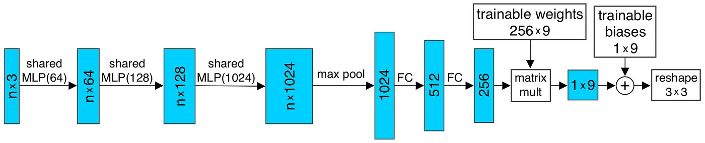

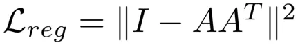
Authors add a regularization term to the matrix “A” which is our T-Net. Do make the learnable weights as an orthogonal matrix, authors add following regularization term:

I’d like to remind some properties of orthogonal matrices and why we are interested in that regularization:

• $A^T A = I$ for all orthogonal matrices
• $det(A) = +/-1$ Basically what it means is our matrix A is invertible and A does nothing to our area/volume or some kind for high-dimensional space than just rotate and/or reflect it. This is a big property for matrices and it is highly desirable. Because we see that: \(<Ax,Ay> = (Ax)^TAy = x^TA^TAy=x^TIy=x^Ty=<x,y>\) This expression tells it mathematically that the transformation under an orthogonal matrix $A$ preserves the angle between two arbitrary vectors $x,y$ and preserves also it’s length. But please keep in mind this does not mean we have $A \in SO(n)$ , since we can only estimate or regularize our matrix to be orthogonal and have no control about $det(A) = 1$.

The regularization term is nothing else then moving our transformation matrix $A$ to be orthogonal so it preserves our area/volume.

# Shared MLP

point_cloud of size (100, 3)

# Shared MLP as nn.Conv1d layer 
shared_mlp = nn.Conv1d(in_channels = 3, out_channels = 64, kernel_size=1)

# weights of shared_mlp are: (64, 3, 1), where every kernel has dims: (3,1)
point_cloud = point_cloud.transpose(-1, -2) # Dims: (3, 100) 

# Pytorch expects: (Batchsize, channels, length) for Conv1d
out = shared_mlp(point_cloud) # Dims: (64, 100)
out = out.transpose(-1, -2) # Dims: (100, 64)

The same layer as shown with pseudo code above can be applied to arbitrary projection sizes of $(C_{in},C_{out})$ (in out case (3,64)). With kernel_size=1 we don’t change our resolution of 100 (same as in images where you apply Conv2d with 1x1 kernel_size only to change the channel dimensions and not the resolution width x height).

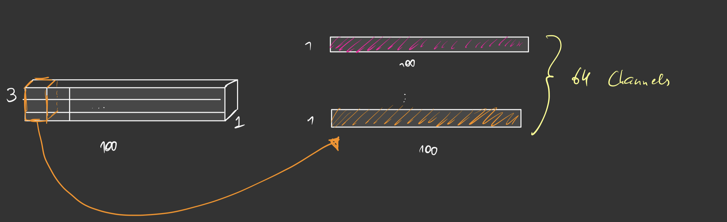
Image above shows how the shared MLP is modeled in PointNet. The kernels of 3x1 are slided across the point clouds. Every point cloud will share the same weights for our kernel/filter so it is shared across multiple points. The same procedure applies to deeper layers.

Limitations of PointNet

One of the limitations PointNet has is it is limited to per-point features and global feature at the end. When we think about Convolutional Neural Network it continuously builds upon receptive field to get higher level information. But it starts with very local low-level semantic information because its receptive field is only lets say 3x3 pixels large. Due to the hierarchical feature learning it can build upon very complex features in the last convolutional layers. But this also means that it will be far more unexplainable and very abstract for us humans. This strategy seems to work very well as seen in Swin-Transformer where the attention modules also builds hierarchically its receptive field (I won’t go further into that).

Another limitation is that the feature learning depends on absolute coordinate. So whenever we have another coordinate system or some transformations to another coordinate system our network will fail because it has (lets say) overfitted or learned the bias of our current configuration.

Another problem of raw point clouds is the fact that a scene in autonomous driving setting has over ~100k points. It is extremely memory inefficient and sparse to use point clouds. Those limitations are tackled by PointNet++.

PointNet++

Authors state that the motivation were drawn from the success of convolutional neural network. As mentioned above, PointNet only extracts per-point features and at the end aggregate with max-pooling the global feature vector of all points. But still local structures are very important for hierarchically building more complex and abstract features to describe the geometric point cloud. “A CNN takes data defined on a regular grid as the input and is able to progressively capture features at increasingly larger scales along a multi-resolution hierarchy”. Basically what is meant is that our receptive field gets progressively larger and our different channels are able to capture extreme complex features. How to define overlapping areas in point clouds was challenging because one could build a k-nearest neighbor ball but won’t be overlapping as in the case of CNN’s.

Authors of PointNet++ leverage farthest point sampling (FPS) to evenly cover the whole set of points. In the image below we see how PointNet++ differs from PointNet. It leverages those Set Abstraction (SA) layers to progressively make larger receptive fields.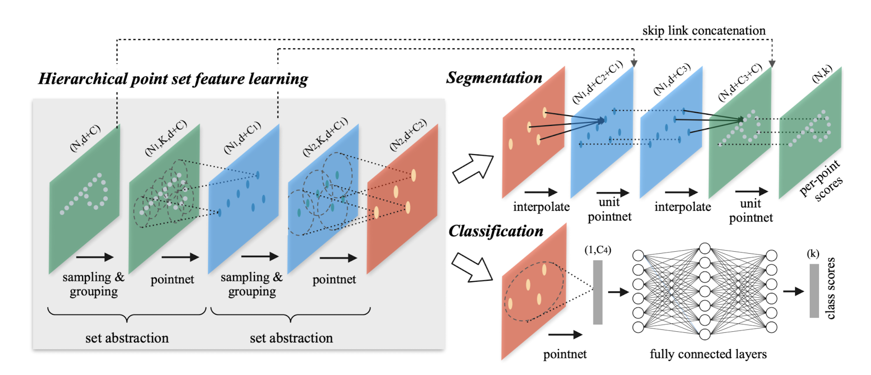

The sampling layer consists of iterative farthest point sampling. Because it is iterative, it is not parallelizable. This makes FPS in PointNet++ a bottleneck for real-time applications like robotics or autonomous driving.

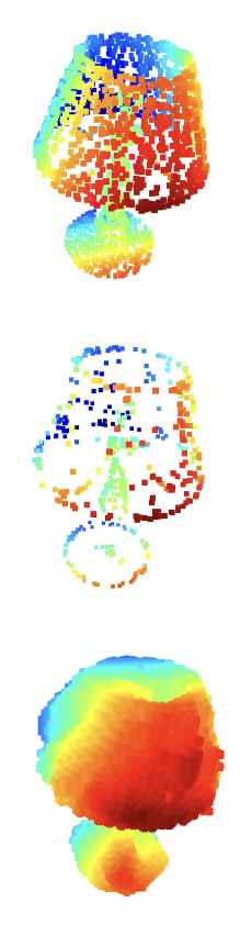
The picture below shows a point cloud of a table taken from the dataset ShapeNet. The original size of the point cloud is [2746, 3]. With FPS we could subsample the farthest points which resulted in a size of [300, 3]. We can choose arbitrary sizes of subsampled points, leading to [N, 3] dimensional output where N=300 in our case.

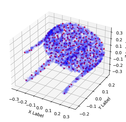
Those 300 points seen in red are the ones selected by the iterative farthest point sampling. It provides a more uniform distribution than randomly sampling points from the point cloud because the region with high dense points within will be overrepresented and those with sparse points underrepresented, leading to poor generalization and feature capturing.

After finding the centroids of our subsampled point cloud, we’ll need to run the points through a ball query layer. It groups all points within a certain radius from the centroid together leading to a dimension of [300, K, 3] where K is our upper limit for points sampled within a point region/radius. Note that every point within the point region is normalized by its centroid. In that sense we will learn features independent of the settings or coordinate system we used in the training set.

Those subsampled points with [300, K, 3] dimension are fed through a pointnet layer. This will take the input permuted as [3, K, 300] and feed it to a 2d convolution with kernel_size = 1x1. As you remember, this won’t change the resolution of the tensor, but only the channel dimension of size 3 to a arbitrary size C leading to an output of [C, K, 300]. The last operation in the pointnet layer is to aggregate global features within the region K. As in PointNet it is done by a max pooling operation w.r.t. to K points within the 300 centroids. The output of the pointnet layer is [300, C].

Those operations above will be repeated hierarchically to achieve the local feature learning in PointNet++. I won’t go in detail through the segmentation and classification branch as it is a normal procedure as in 2D perception.

The main drawbacks of point-based 3D learning are the following:

• FPS is restricted by iteratively capturing new centroids, so it is not parallelizable
• Increasing the number of centroids will lead to a finer point cloud and thus more representation power in the feature learning, but we will also be increasing the memory consumption
• The context radius is critical. If radius is large we will be loosing fine-grained 3d information, radius too small, we will loose local feature learning and collapsing in PointNet instead of PointNet++.

3D Deep Learning on voxels

To extend the approach of 2D convolutions to 3D is not a very complex task. All the layers such as MaxPool, Activation Functions, BatchNorm, Global Average Pooling etc. do work the same way as in 2D images but extended to volumes. So you’ll have to define kernel volumes instead of kernel windows for example.

But there is one problem with this approach: the sparsity in the 3d space with voxelization is extremely large. There is the tradeoff: If you choose very large voxel size, lets say 20cm, you’ll end up with less zero-voxels (I am referring to a voxel which is empty as zero-voxel for convenience) but you’ll loose also information due to the quantization. If you choose a voxel size which is more fine-grained, then you’ll end up with much more zero-voxels but you’ll have a more fine-grained representation of the scene.

Nonetheless one has an extremely large amount of zero-voxels in the representation. But if not modelled correctly, you’ll end up sliding your convolutional filter over the grid and still calculating the outputs although you know there are empty.

There is another way to do that and its called sparse convolutions. SECOND is a seminal work in that direction, which is used for 3d object detection. The procedure starts with preallocating the number of maximum voxels allowed in the scene. Secondly, it voxelizes the 3d point clouds and saves the results in a hash table. “If the voxel related to a point does not yet exist, we set the corresponding value in the hash table, otherwise we increment the number of voxels by one”.

# VOXEL Features and Coordinates 
for point in point_cloud: 
	voxel = voxelize(point) # assigns point to corresponding voxel
	if hash_table[voxel]: 
		hash_table[voxel] += 1
		voxel_num += 1
	else: 
		hash_table[voxel] = 0
	if voxel_num >= max_voxels: 
		break 

for voxel, num_points_per_voxel in hash_table.items(): 
	# get voxel and (voxel_coordinates, num_points_per_voxel) as features

The VFE is adopted from VoxelNet: End-to-End Learning for Point Cloud based 3D Object. As mentioned earlier, point cloud coming from sensors like LiDAR typically are composed of ~100k points, so to process all of them is extremely memory and computationally inefficient. So in order to also decrease the so called “density bias” in point clouds, the layer applies Random Sampling. The number of points to sample is predefined and is a hyperparameter. So every voxel which has more than $T$ points will be sampled randomly. Per authors the sampling strategy has two advantages: 1) computational savings and 2) decreases the imbalance of points between the voxels. The Voxel Feature Encoding Layer employs a hierarchical feature learning strategy which was discussed before, similar to CNN’s. A set of Voxels is denoted as $V={ p_i = [x_i, y_i, z_i, r_i]^T \in \mathbb{R}^4}_{i=1,…,t}$ ,in other words $V$ is just one voxel consisting of $t \leq T$ points. So one voxel has maximum T number of points in it, where $x,y,z$ are the coordinates of the point and $r$ is the reflectance feature. The next step is to compute the voxel-wise mean of $V$ as $(v_x, v_y,v_z)$ . To overcome the above mentioned bias of the absolute coordinate system each point within the voxel is subtracted by the mean of all the points in the voxel $V$. The pseudo code for generating point features is shown below:

# Voxel Feature Extraction
for voxel in voxel_set: 
	points_per_voxel = []
	for point in voxel: 
		points_per_voxel.append(point)

	points_per_voxel = np.array(points_per_voxel) # Dims: (t, 4)
	# reflectance is not included 
	points_mean = np.mean(points_per_voxel[:,:3] axis = 0) 
	points_per_voxel_mean = points_per_voxel[:, :3] - points_mean 

	# features of size: (t, 7)
	points_features = np.concatenate(points_per_voxel, points_per_voxel_mean)


	# FCN is for example nn.Linear(7, 32)
	f_i = FCN(points_feautures) # Dims: (t, 32)
	f_i_tilde, _ = torch.max(f_i, dim=-2, keepdim=True) # Dims: (1, 32)
	f_i_tilde = f_i_tilde.repeat(t, 1) # Dims: (100, 32)

	out = torch.concat([f_i, f_i_tilde], dim=-1) # Dims: (100, 64)

The points_features are then fed to a fully connected network which consists of linear layer, batch norm and ReLU. The output of the VFE is $f^{out}_i \in \mathbb{R}^{2m}$ where $m$ is the specified output dimension which was in our case 32 but can be chosen arbitrarily. 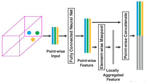Stated by the authors of VoxelNet: “Because the output feature combines both point-wise features and locally aggregated feature, stacking VFE layers encodes point interactions within a voxel and enables the final feature representation to learn descriptive shape information”. At the end of those VFE-Layers follows a FCN with output size $C$. At the end of the “Feature Learning Network” we obtain a sparse tensor of dimensions $(C\times D \times H \times W)$ where D, H, W are the ranges along the z,y,x axis respectively.
SECOND integrates submanifold sparse convolutions after Voxel Feature Extraction. Submanifold sparse convolutions differ from sparse convolution in the following:

Sparse convolutions keep a hash table of the voxels which are non-empty to calculate some convolutions to the output. When we take a look at the receptive field of 2d Convs we’ll see that the receptive field grows with the depth of the network. The exact formula for calculating the receptive field is given as follows \(r_0 = \sum^{L}_{l=1} \Biggl( (k_l -1) \prod_{i=1}^{l-1} s_i\Biggr) + 1\) Where $k$ is kernel size, $s$ is the stride and $l$ are the layers. For example for two layers with kernel_size = 3 and stride = 1, our receptive field is 5x5 pixels in the original image. Image shown below.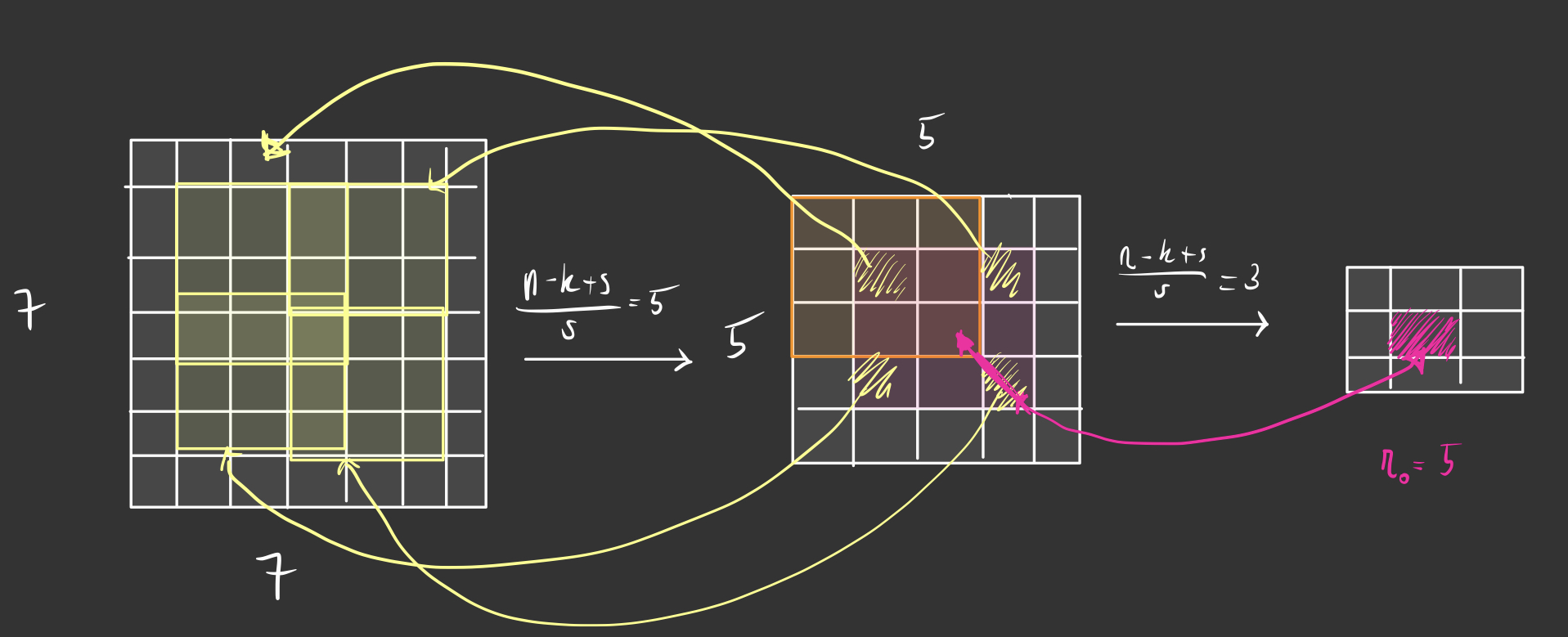

If we are using a padding of one, our receptive field would still 5x5 but now our input would be the same size as the output. The conclusion of the authors in https://arxiv.org/pdf/1706.01307.pdf stated that regular convolutions substantially reduce the sparsity of the feature maps because we hierarchically get more activated pixels in our resolution once we get deeper in our layers. In images this might not be a problem but when you are dealing with a lot of zero-voxels your unnecessary computation gets a lot worse once your zero-voxels get non-zero because of the receptive field of also 3D convolutions.

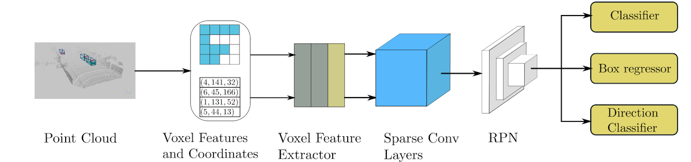
As the figure below depicts, sparse conv layers are followed after VFE layers explained above. Per authors, the middle layer is used to learn information about the z-axis. It will incrementally downsample the z-dimension ending with a so called “Birds Eye View” where we have z=1 and only top-down view of the scene.

After converting the 3D data to a BEV map, the procedure of RPN is similar to Faster R-CNN where region proposals are learned seperately, making this approach a Two-Stage detector.

Point-Voxel Approaches

PV-based approaches combine the positive aspects of both worlds. The paper “Point-Voxel CNN For Efficient 3D Deep Learning” introduces the idea. The motivation was the following:

• Point-based approaches (like PointNet etc.) are extremely memory efficient due to the sparsity of the point cloud. Because raw points are sparse they use $random$ $memory$ $access$. Another disadvantage is they come in domains like AD with over 100k points per scene
• Point-based approaches on the other hand are fast.
• Voxel-based approached (like VoxelNet etc.) are regularly sampled data same as grid. They don’t suffer from random memory access. What they struggle with is the large memory footprint. If the voxel-size / resolution is low, a lot of information is lost. When the resolution is high, the memory it takes is huge. The space complexity is $O(N^3)$.

Authors claim that PV-CNN outperforms voxel-based baseline with 10x lower memory consumption and achieves 7x speedup compared to point-based approaches.

The network is divided into two branches: point-based branch and voxel-based branch. Let us dive into the different branches and how they work.

Basically the point-based branch works very similar to PointNet/PointNet++. They make use of shared MLP’s as in PointNet with 1-dimensional conv layers to learn per point features. They make also use of Set-Abstraction Layer (PointNet++: Sampling+Grouping+PointNet Layer). This will map the point clouds to a higher dimensional feature space.

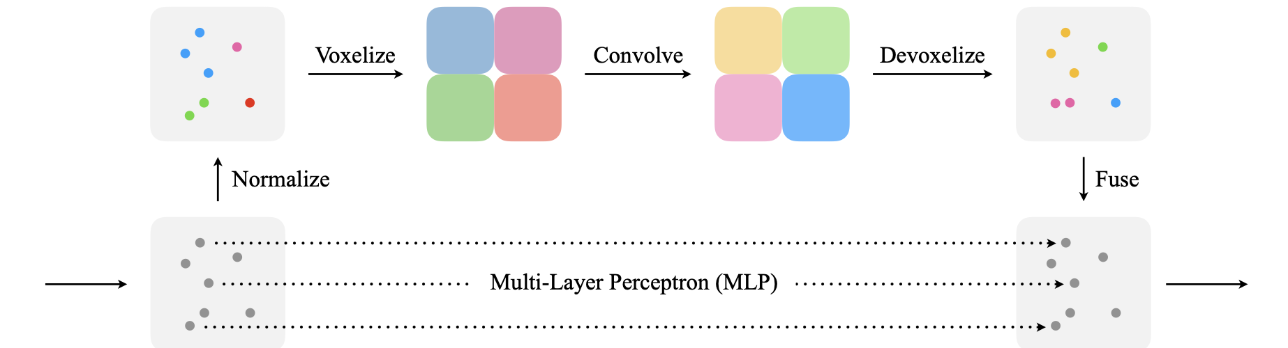
The voxel-branch is quite novel. The input to the branch is a tuple of ${p_k, f_k }$ where $p_k$ is the $(x_k, y_k, z_k)$ coordinates of point cloud and $f_k$ is the feature of point cloud. The procedure is as followed:

• Normalization: First the coordinates of the point cloud are normalized with the voxel center as the origin to overcome special settings and generalize to arbitrary coordinate systems. The output of the Normalization layer is ${\hat{p_k}, f_k }$ where $\hat{p_k}$ are the normalized coordinates of the point cloud. Note here: the features are not normalized and kept the same.
• Voxelization: the voxelization is done as normally. Out of the voxelization step we get also voxel features and coordinates. The voxel features are the normalized features of all points falling into the voxel. The dimensions should be [f_k, u, v, w] where u,v,w are the voxel dimensions.
• Convolve: Is a typical layer of 3D convolutions stacked on top. Authors apply CBR (convolution-batch_norm-relu).
• Devoxelization: To be able to fuse the two branches together, it is important to convert the voxels to point clouds. The coordinates of the different points are given as $\hat{p_k}$. What we need to devoxelize are the learned features of the voxels. One naive approach could be to use the voxel-feature to all points within the voxels. This will neglect the unique features of the points and make them have the same features. Instead Authors suggest to use trilinear interpolation to interpolate the features to the points $p_k$ to have distinct features.

Picture below shows the proposed PVConv Layer.

PVConv Layers can be inserted into existing architectures like PointNet where you could replace the MLP layers with PVConv layers.

Those were the most promising 3d deep learning models for perception of autonomous systems.

Those were the most promising 3d deep learning models for perception of autonomous systems.